Understanding the Equation for Covariance
📋 In this guide
The equation for covariance is a fundamental concept in statistics that measures the degree to which two variables change together. This mathematical tool is essential for understanding relationships between datasets, making it a crucial topic for students tackling statistics courses. However, many students find the equation for covariance challenging, primarily because it requires a solid grasp of statistical concepts and algebra equations. In this article, we will demystify this topic, providing a clear, step-by-step guide to understanding and applying the equation for covariance.
By the end of this article, you'll understand not only the equation for covariance but also how to apply it to real-world problems. We'll walk you through the definition, break down the steps involved in its calculation, and provide detailed examples that illustrate its application. Along the way, we'll highlight common mistakes to avoid and discuss practical applications in various fields. Whether you're grappling with mystatlab homework answers statistics or wondering which regression equation best fits the data, this guide will equip you with the knowledge you need.
Understanding covariance is not just about crunching numbers; it involves interpreting data and drawing meaningful conclusions from it. This article aims to bridge the gap between theory and practice, making the equation for covariance accessible to everyone, from high school students to professionals in data-driven fields. So, let's dive in and explore the intricacies of the equation for covariance, ensuring you have the tools to tackle your statistical challenges with confidence.
Step-by-Step: How to Solve Equation For Covariance
Step 1: Calculate the Mean of Each Dataset
The first step in computing the equation for covariance is to determine the mean of each dataset. The mean is simply the average value of the data points. To find the mean of a dataset X, add all the values in X and divide by the number of values. Repeat this process for dataset Y. For example, if X = [2, 4, 6], the mean of X would be (2 + 4 + 6) / 3 = 4. Similarly, calculate the mean for dataset Y.
Step 2: Determine Deviations from the Mean
Once you have the means for both datasets, the next step is to calculate the deviation of each data point from its respective mean. Subtract the mean of X from each value in X to get the deviations for dataset X. Do the same for dataset Y. These deviations represent how much each data point varies from the average. This step is crucial because it sets the stage for measuring how these variations correlate between the two datasets.
Step 3: Multiply Deviations and Sum the Products
After calculating the deviations, multiply the deviation of each data point in X by the corresponding deviation in Y. This multiplication will give you the product of deviations for each pair of data points. Once you have these products, sum them up. This sum represents the combined variance between the two datasets and is a critical component of the equation for covariance.
Step 4: Divide by the Number of Data Points Minus One
The final step is to divide the sum of the products of deviations by the number of data points minus one (n - 1). This division provides the average covariance between the datasets. The reason for subtracting one from the number of data points is to account for the degrees of freedom in the dataset, ensuring an unbiased estimate of covariance. The result is the covariance value, which can be positive, negative, or zero, indicating the direction and strength of the relationship between the datasets.
🤖 Stuck on a math problem?
Take a screenshot and let our AI solve it step-by-step in seconds
⚡ Try MathSolver Free →Worked Examples
Example 1
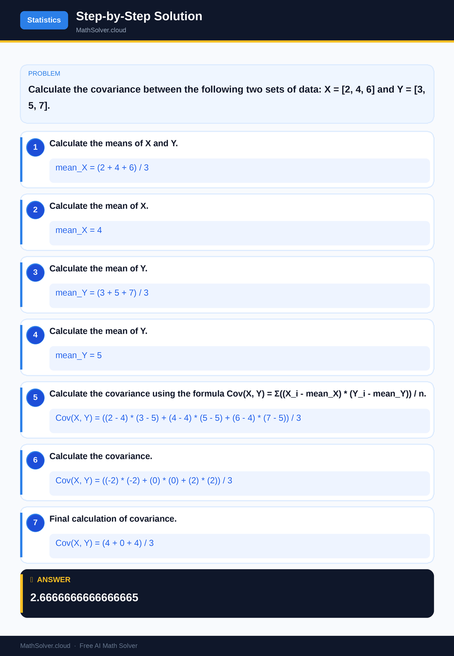
MathSolver Chrome extension solving this problem step-by-step
Example 2
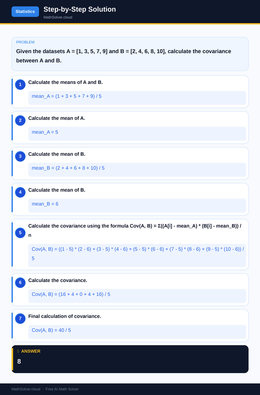
MathSolver Chrome extension solving this problem step-by-step
Common Mistakes to Avoid
One common mistake students make when calculating the equation for covariance is failing to subtract the means correctly, leading to inaccurate deviations. Always double-check that you subtract the mean of each dataset from its respective data points. Another frequent error is incorrectly calculating the sum of the products of deviations. Ensure each step is followed methodically to avoid arithmetic errors. Finally, remember to divide by n - 1 rather than n; this adjustment for degrees of freedom is crucial for an unbiased result.
Real-World Applications
The equation for covariance is widely used in finance to assess the relationship between asset returns. For instance, investors analyze the covariance between stock returns to diversify their portfolios effectively. A positive covariance indicates that stocks move together, while a negative covariance suggests they move inversely, aiding in risk management. In meteorology, covariance can help assess the relationship between temperature and humidity levels, crucial for weather prediction models.
In manufacturing, understanding the covariance between different production variables can optimize processes and improve efficiency. By examining how variables like temperature and pressure interact, manufacturers can fine-tune production to increase yield and reduce waste. These real-world applications highlight the equation for covariance's importance across diverse fields, demonstrating its utility beyond the classroom.
Frequently Asked Questions
❓ What does the equation for covariance tell us?
❓ Why is the equation for covariance important in statistics?
❓ How can AI help with the equation for covariance?
❓ How is covariance different from correlation?
❓ What are the limitations of using the equation for covariance?
🚀 Solve any math problem instantly
2,000+ students use MathSolver every day — join them for free
📥 Add to Chrome — It's Free