Mastering Stochastic Differential Equations
📋 In this guide
Stochastic differential equations are a fascinating and complex area of mathematics that combines the unpredictability of random processes with the precision of calculus. These equations are often encountered in fields like finance, physics, and engineering, where systems are influenced by random variability. However, students frequently struggle with stochastic differential equations due to their abstract nature and the mathematical rigor required to understand them. Throughout this article, you'll gain a comprehensive understanding of stochastic differential equations, learn how to solve them step-by-step, and discover their real-world applications.
The intrinsic complexity of stochastic differential equations arises from the inclusion of stochastic processes—random variables that evolve over time. This makes them fundamentally different from ordinary differential equations, which typically deal with deterministic systems. As we delve into this topic, you'll learn about key concepts such as Wiener processes and Ito calculus, which are essential for mastering stochastic differential equations. By the end of this article, you should feel more confident in tackling problems involving these equations and appreciating their role in modeling random systems.
In this article, you'll also discover the concept of score-based generative modeling through stochastic differential equations, an exciting application in the field of artificial intelligence. You'll see how methods like the Oksendal stochastic differential equations approach can be used to solve complex problems. Whether you're a student trying to wrap your head around these equations or a professional looking to apply them in your work, this detailed guide will provide valuable insights and practical solutions.
Step-by-Step: How to Solve Stochastic Differential Equations
Step 1: Understanding the Basics
Before diving into solving stochastic differential equations, it’s crucial to understand the fundamental components. First, familiarize yourself with the standard Wiener process, denoted as W(t). It represents a continuous-time stochastic process with independent and normally distributed increments. The process starts at zero, and its variance grows linearly with time. Understanding the behavior of W(t) is essential, as it forms the backbone of the stochastic part of the equation. Next, recognize the role of the drift term, f(X(t), t), which represents the deterministic component influencing the rate of change of the process. The diffusion term, g(X(t), t), represents the random component and is crucial for modeling the system's volatility.
Step 2: Setting Up the Equation
Once you understand the components, the next step is to set up your stochastic differential equation properly. Begin by identifying the variables involved and specifying the initial conditions. For instance, determine the initial value of the process, X(0). Then, identify the drift and diffusion coefficients based on the problem context. Ensure these coefficients make sense in terms of units and dimensions. The proper setup allows you to translate a real-world problem into a mathematical model accurately. This step is critical because any misinterpretation of the problem can lead to incorrect modeling and solutions.
Step 3: Applying Ito's Lemma
Ito's Lemma is a fundamental tool in solving stochastic differential equations, akin to the chain rule in calculus for deterministic functions. It provides a method for finding the differential of a function of a stochastic process. If you have a function F(X(t), t), Ito's Lemma helps express dF in terms of dX(t) and dt. Applying Ito's Lemma involves calculating partial derivatives of F with respect to both X and t, and incorporating these into the equation. This step is often where students struggle, but with practice, it becomes a powerful technique for simplifying and solving SDEs.
Step 4: Solving the Equation
With the equation set up and Ito's Lemma applied, the final step is solving the stochastic differential equation. This often involves integrating both sides of the equation over time. The solution may require numerical methods, especially for complex SDEs without closed-form solutions. When dealing with simpler equations, analytical methods can be applied to find explicit solutions. Verify your results by checking the consistency of the solution with the initial conditions and problem context. Solutions to stochastic differential equations often involve expectations, variances, or distributions, so interpret these results in the context of the problem.
🤖 Stuck on a math problem?
Take a screenshot and let our AI solve it step-by-step in seconds
⚡ Try MathSolver Free →Worked Examples
Example 1
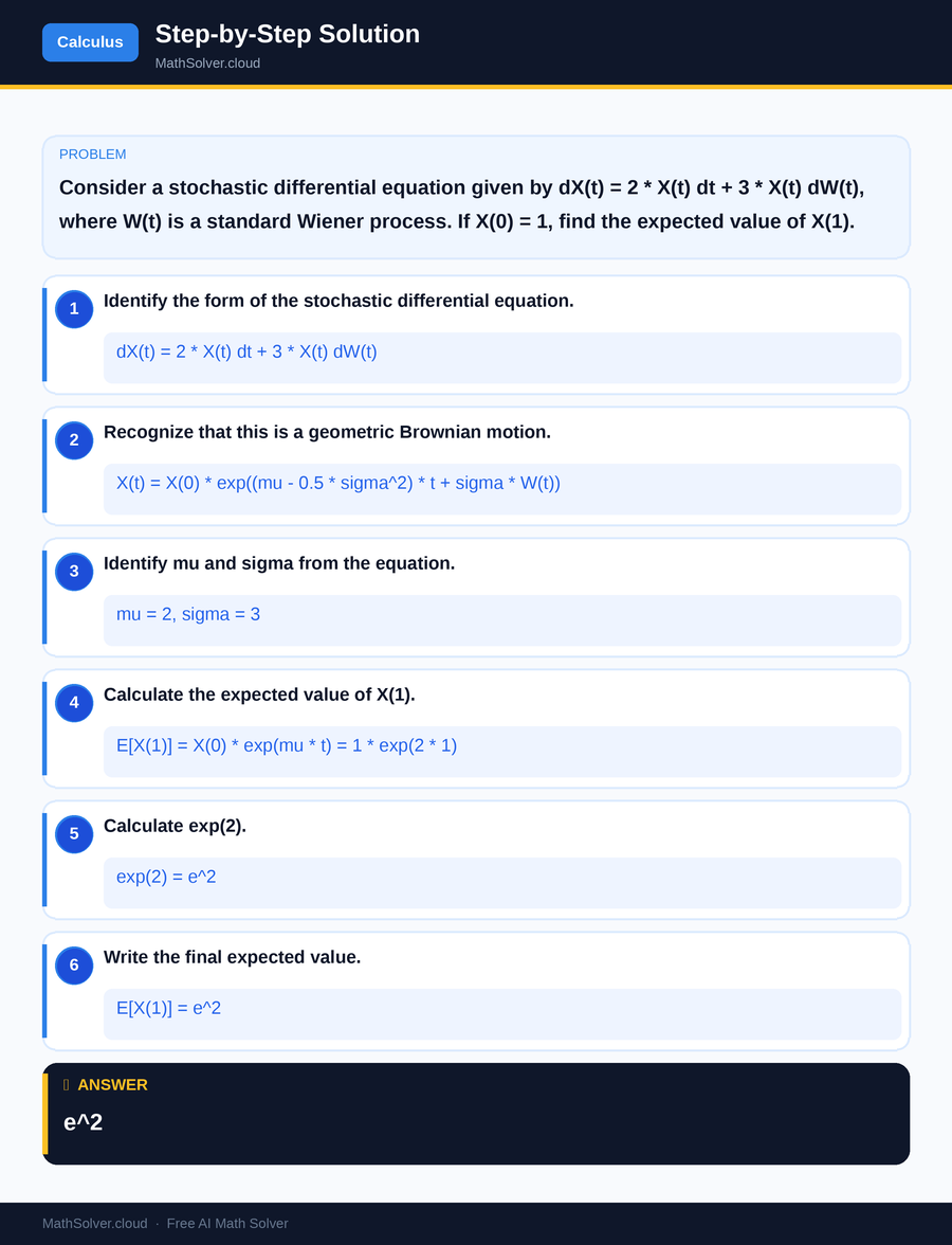
MathSolver Chrome extension solving this problem step-by-step
Example 2
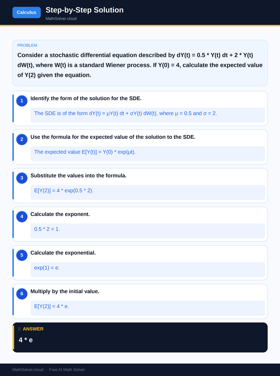
MathSolver Chrome extension solving this problem step-by-step
Common Mistakes to Avoid
One common mistake students make is misunderstanding the role of the Wiener process. It's crucial to remember that W(t) represents a random process with specific properties, not just a simple variable. Misinterpreting this can lead to incorrect solutions. Another frequent error is neglecting to apply Ito's Lemma correctly. It's essential to practice this technique and understand its derivation to avoid mistakes.
Students also often forget to verify their solutions against the initial conditions and the context of the problem. Always double-check that your solution is consistent with the given conditions and makes sense in real-world applications. Ensuring that your mathematical model accurately represents the problem context is vital for obtaining correct and meaningful results.
Real-World Applications
Stochastic differential equations are widely used in finance, particularly in modeling stock prices and interest rates. The famous Black-Scholes model, which is used for option pricing, is based on a stochastic differential equation. Understanding these equations is essential for professionals working in financial engineering and risk management.
In physics, stochastic differential equations model systems with inherent randomness, such as the motion of particles suspended in fluid (Brownian motion). Engineers also use these equations to model noise in electronic circuits and to simulate random processes in control systems. These real-world applications underscore the importance of mastering stochastic differential equations for students and professionals alike.
Frequently Asked Questions
❓ What are stochastic differential equations?
❓ Why are stochastic differential equations challenging for students?
❓ How can AI help with stochastic differential equations?
❓ What is score-based generative modeling through stochastic differential equations?
❓ How can I avoid common mistakes when solving stochastic differential equations?
🚀 Solve any math problem instantly
2,000+ students use MathSolver every day — join them for free
📥 Add to Chrome — It's Free