Exploring the World of Differential Equations
📋 In this guide
Differential equations are a fundamental aspect of calculus and mathematical modeling, forming the backbone of various scientific and engineering disciplines. They describe how a particular quantity changes in relation to another, often involving rates of change. Despite their importance, many students find differential equations challenging due to their abstract nature and the intricate problem-solving skills required. This article will delve into the world of differential equations, providing a comprehensive understanding and equipping you with the tools to tackle these problems with confidence. By the end of this article, you will gain insights into different types of differential equations, learn step-by-step problem-solving techniques, and explore real-world applications that highlight their significance.
Differential equations can be intimidating due to the complex mathematical concepts they encompass. From ordinary differential equations to partial differential equations and even stochastic differential equations, each type presents its own unique set of challenges. Understanding the differences and knowing the appropriate methods to solve them is crucial for success in courses like AP Calculus BC and beyond. This guide will help demystify these concepts, offering clarity and practical examples to bolster your confidence.
In addition to theoretical knowledge, this article introduces digital tools such as differential equations calculators. These calculators can simplify the solving process and provide instant solutions to complex problems. We'll also explore how AI-driven platforms, such as MathSolver cloud, can assist in understanding and solving differential equations through interactive and user-friendly interfaces. By the end, you'll not only understand differential equations better but also appreciate their applications in fields like physics, engineering, and finance.
Step-by-Step: How to Solve Differential Equations
Step 1: Identifying the Type of Differential Equation
The first step in solving a differential equation is to identify its type. Differential equations are broadly classified into ordinary differential equations and partial differential equations. Ordinary differential equations involve functions of a single variable and their derivatives, whereas partial differential equations involve functions of multiple variables and their partial derivatives. Identifying the type is crucial because it dictates the methods you will use to solve the equation. For instance, linear differential equations have a standard form and solution techniques, while nonlinear equations might require specific methods or numerical approaches.
Step 2: Determining the Order and Degree
The next step involves determining the order and degree of the differential equation. The order of a differential equation is the highest derivative present in the equation. For example, in the equation d^2y/dx^2 - 4dy/dx + 4y = 0, the order is two because the highest derivative is the second derivative. The degree is the power of the highest derivative, provided the equation is polynomial in its derivatives. Knowing the order and degree helps in choosing the right solution method, such as separation of variables for first-order equations or the characteristic equation for higher-order linear equations.
Step 3: Choosing the Solution Method
Once the differential equation's type, order, and degree are identified, the next step is to choose an appropriate method for solving it. For first-order ordinary differential equations, methods such as separation of variables, integrating factors, or exact equations are commonly used. For higher-order linear differential equations, the characteristic equation approach is often employed. In the case of partial differential equations, methods like separation of variables or transform methods may be applicable. The chosen method should simplify the equation to a form where the unknown function can be easily determined.
Step 4: Solving and Verifying the Solution
After applying the appropriate method, solve the equation to find the unknown function. Verification is a crucial part of this step. Substitute the solution back into the original differential equation to ensure it satisfies the equation for the given conditions. For example, if you have an initial value problem, check that the solution meets the initial conditions provided. This step confirms the correctness of your solution and ensures that no errors were made in the process.
🤖 Stuck on a math problem?
Take a screenshot and let our AI solve it step-by-step in seconds
⚡ Try MathSolver Free →Worked Examples
Example 1
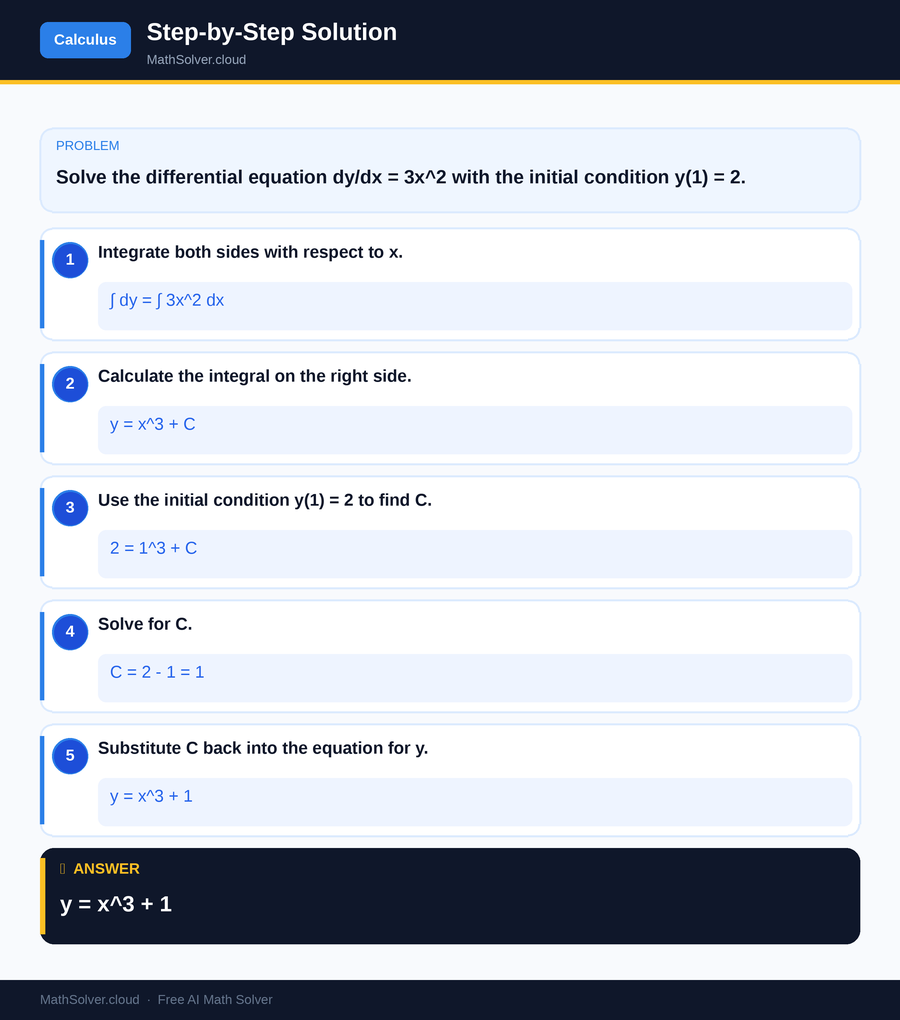
MathSolver Chrome extension solving this problem step-by-step
Example 2
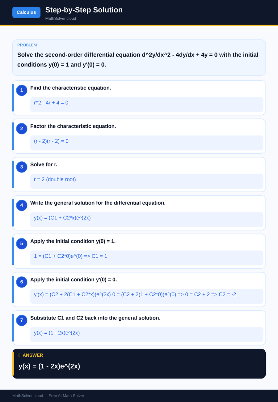
MathSolver Chrome extension solving this problem step-by-step
Common Mistakes to Avoid
One common mistake students make is failing to correctly identify the type and order of the differential equation, leading to the application of incorrect solution methods. It's crucial to carefully analyze the equation's structure before proceeding with the solving method.
Another frequent error is neglecting to verify the solution. After solving the differential equation, always substitute your solution back into the original equation to ensure it satisfies all given conditions, including initial or boundary conditions.
Students also often confuse the roles of constants of integration in their solutions. When solving differential equations, particularly those involving initial or boundary conditions, it's essential to properly determine these constants to ensure the solution is complete and accurate. Miscalculating these constants can lead to incorrect solutions that do not meet the specified conditions.
Real-World Applications
Differential equations have a wide array of real-world applications, allowing us to model and analyze various phenomena. In physics, they are crucial in describing motion and forces, such as in Newton's laws of motion. Engineers use differential equations to model and predict system behaviors, such as electrical circuits and structural analysis. In biology, they help model population dynamics and the spread of diseases.
One fascinating application is in financial mathematics, where stochastic differential equations are used to model stock prices and market trends. These equations help in the development of strategies for asset pricing and risk management. Another interesting application is in score-based generative modeling through stochastic differential equations, which is a technique used in machine learning to generate data with specific statistical properties.
Frequently Asked Questions
❓ What are differential equations?
❓ Why do students struggle with differential equations?
❓ How can AI help with differential equations?
❓ What is the difference between ordinary and partial differential equations?
❓ How can I verify my solution to a differential equation?
🚀 Solve any math problem instantly
2,000+ students use MathSolver every day — join them for free
📥 Add to Chrome — It's Free